The task of estimating the number of distinct values (DVs) in a large dataset arises in a wide variety of settings in computer science and elsewhere. We provide DV estimation techniques for the case in which the dataset of interest is split into partitions. We create for each partition a synopsis that can be used to estimate the number of DVs in the partition. By combining and extending a number of results in the literature, we obtain both suitable synopses and DV estimators. The synopses can be created in parallel, and can be easily combined to yield synopses and DV estimates for “compound” partitions that are created from the base partitions via arbitrary multiset union, intersection, or difference operations. Our synopses can also handle deletions of individual partition elements. We prove that our DV estimators are unbiased, provide error bounds, and show how to select synopsis sizes in order to achieve a desired estimation accuracy. Experiments and theory indicate that our synopses and estimators lead to lower computational costs and more accurate DV estimates than previous approaches.
1. Introduction
The task of determining the number of distinct values (DVs) in a large dataset arises in a wide variety of settings. One classical application is population biology, where the goal is to determine the number of distinct species, based on observations of many individual animals. In computer science, applications include network monitoring, document search, predicate-selectivity estimation for database query optimization, storage-size estimation for physical database design, and discovery of metadata features such as keys and duplicates.
The number of DVs can be computed exactly by sorting the dataset and then executing a straightforward scan-and-count pass over the data; alternatively, a hash table can be constructed and used to compute the number of DVs. Neither of these approaches scales well to the massive datasets often encountered in practice, because of heavy time and memory requirements. A great deal of research over the past 25 years has therefore focused on scalable approximate methods. These methods work either by drawing a random sample of the data items and statistically extrapolating the number of DVs, or by taking a single pass through the data and using hashing techniques to compute an estimate using a small, bounded amount of memory.
Almost all of this work has focused on producing a given synopsis of the dataset, such as a random sample or bit vector, and then using the synopsis to obtain a DV estimate. Issues related to combining and exploiting synopses in the presence of union, intersection, and difference operations on multiple datasets have been largely unexplored, as has the problem of handling deletions of items from the dataset. Such issues are the focus of this paper, which is about DV estimation methods when the dataset of interest is split into disjoint partitions, i.e., disjoint multisets.a The idea is to create a synopsis for each partition so that (i) the synopsis can be used to estimate the number of DVs in the partition and (ii) the synopses can be combined to create synopses for “compound” partitions that are created from the base partitions using multiset union, intersection, or difference operations.
This approach permits parallel processing, and hence scalability of the DV-estimation task to massive datasets, as well as flexible processing of DV-estimation queries and graceful handling of fluctuating data-arrival rates. The partitioning approach can also be used to support automated data integration by discovering relationships between partitions. For example, suppose that the data is partitioned by its source: Amazon customers versus YouTube downloaders. Then DV estimates can be used to help discover subset-inclusion and functional-dependency relationships, as well as to approximate the Jaccard distance or other similarity metrics between the domains of two partitions; see Brown and Haas and Dasu et al.4,6
Our goal is therefore to provide “partition-aware” synopses for DV estimation, as well as corresponding DV estimators that exploit these synopses. We also strive to maintain the best possible accuracy in our DV estimates, especially when the size of the synopsis is small: as discussed in the sequel, the size of the synopsis for a compound partition is limited by the size of the smallest input synopsis.
We bring together a variety of ideas from the literature to obtain a solution to our problem, resulting in best-of-breed DV estimation methods that can also handle multiset operations and deletions. We first consider, in Section 2, a simple “KMV” (K Minimum hash Values) synopsis2 for a single partition—obtained by hashing the DVs in the partition and recording the K smallest hash values—along with a “basic” DV estimator based on the synopsis; see Equation 1. In Section 3, we briefly review prior work and show that virtually all prior DV estimators can be viewed as versions of, or approximations to, the basic estimator. In Section 4, we propose a new DV estimator—see Equation 2—that improves upon the basic estimator. The new estimator also uses the KMV synopsis and is a deceptively simple modification of the basic estimator. Under a probabilistic model of hashing, we show that the new estimator is unbiased and has lower mean-squared error than the basic estimator. Moreover, when there are many DVs and the synopsis size is large, we show that the new unbiased estimator has essentially the minimal possible variance of any DV estimator. To help users assess the precision of specific DV estimates produced by the unbiased estimator, we provide probabilistic error bounds. We also show how to determine appropriate synopsis sizes for achieving a desired error level.
In Section 5, we augment the KMV synopsis with counters—in the spirit of Ganguly et al. and Shukla et al.10,18—to obtain an “AKMV synopsis.” We then provide methods for combining AKMV synopses such that the collection of these synopses is “closed” under multiset operations on the parent partitions. The AKMV synopsis can also handle deletions of individual partition elements. We also show how to extend our simple unbiased estimator to exploit the AKMV synopsis and provide unbiased estimates in the presence of multiset operations, obtaining an unbiased estimate of Jaccard distance in the process; see Equations 7 and 8. Section 6 concerns some recent complements to, and extensions of, our original results in Beyer et al.3
2. A Basic Estimator and Synopsis
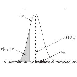
The idea behind virtually all DV estimators can be viewed as follows. Each of the D DVs in a dataset is mapped to a random location on the unit interval, and we look at the position U(k) of the kth point from the left, for some fixed value of k; see Figure 1. The larger the value of D, i.e., the greater the number of points on the unit interval, the smaller the value of U(k). Thus D can plausibly be estimated by a decreasing function of U(k).
Specifically, if D
 1 points are placed randomly and uniformly on the unit interval, then, by symmetry, the expected distance between any two neighboring points is 1/(D + 1)
 1/D, so that the expected value of U(k), the kth smallest point, is E[U(k)
Σkj=1 (1/D) = k/D. Thus D
k/E[U(k)]. The simplest estimator of E[U(k)] is simply U(k) itself—the so-called “method-of-moments” estimator—and yields the basic estimator
1/D, so that the expected value of U(k), the kth smallest point, is E[U(k)
Σkj=1 (1/D) = k/D. Thus D
k/E[U(k)]. The simplest estimator of E[U(k)] is simply U(k) itself—the so-called “method-of-moments” estimator—and yields the basic estimator

The above 1-to-1 mapping from the D DVs to a set of D uniform random numbers can be constructed perfectly using O(D log D) memory, but this memory requirement is clearly infeasible for very large datasets. Fortunately, a hash function—which typically only requires an amount of memory logarithmic in D—often “looks like” a uniform random number generator. In particular, let
 (A) = {v1, v2, …, vD} be the domain of multiset A, i.e., the set of DVs in A, and let h be a hash function from
(A) to {0, 1, …, M}, where M is a large positive integer. For many hash functions, the sequence h(v1), h(v2), …, h(vD) looks like the realization of a sequence of independent and identically distributed (i.i.d.) samples from the discrete uniform distribution on {0, 1, …, M}. Provided that M is sufficiently greater than D, the sequence U1 = h(v1)/M, U2 = h(v2)/M, …, UD = h(vD)/M will approximate the realization of a sequence of i.i.d. samples from the continuous uniform distribution on [0, 1]. This assertion requires that M be much larger than D to avoid collisions, i.e., to ensure that, with high probability, h(vi) ≠ h(vj) for all i ≠ j. A “birthday problem” argument 16, p. 45 shows that collisions will be avoided when M = Ω(D2). We assume henceforth that, for all practical purposes, any hash function that arises in our discussion avoids collisions. We use the term “looks like” in an empirical sense, which suffices for applications. Thus, in practice, the estimator
(A) = {v1, v2, …, vD} be the domain of multiset A, i.e., the set of DVs in A, and let h be a hash function from
(A) to {0, 1, …, M}, where M is a large positive integer. For many hash functions, the sequence h(v1), h(v2), …, h(vD) looks like the realization of a sequence of independent and identically distributed (i.i.d.) samples from the discrete uniform distribution on {0, 1, …, M}. Provided that M is sufficiently greater than D, the sequence U1 = h(v1)/M, U2 = h(v2)/M, …, UD = h(vD)/M will approximate the realization of a sequence of i.i.d. samples from the continuous uniform distribution on [0, 1]. This assertion requires that M be much larger than D to avoid collisions, i.e., to ensure that, with high probability, h(vi) ≠ h(vj) for all i ≠ j. A “birthday problem” argument 16, p. 45 shows that collisions will be avoided when M = Ω(D2). We assume henceforth that, for all practical purposes, any hash function that arises in our discussion avoids collisions. We use the term “looks like” in an empirical sense, which suffices for applications. Thus, in practice, the estimator
 can be applied with U(k) taken as the kth smallest hash value (normalized by a factor of 1/M). In general, E[1/X]> 1/E[X] for a non-negative random variable X,17, p. 351 and hence

i.e., the estimator
is biased upwards for each possible value of D, so that it overestimates D on average. Indeed, it follows from the results in Section 4.1 that E[
]=∞ for k = 1. In Section 4, we provide an unbiased estimator that also has lower mean-squared error than
.
Note that, in a certain sense, the foregoing view of hash functions—as algorithms that effectively place points on the unit interval according to a uniform distribution—represents a worst-case scenario with respect to the basic estimator. To the extent that a hash function spreads points evenly on [0, 1], i.e., without the clumping that is a byproduct of randomness, the estimator
will yield more accurate estimates. We have observed this phenomenon experimentally.3
The foregoing discussion of the basic estimator immediately implies a choice of synopsis for a partition A. Using a hash function as above, hash all of the DVs in A and then record the k smallest hash values. We call this synopsis a KMV synopsis (for k minimum values). The KMV synopsis can be viewed as originating in Bar-Yossef et al.,2 but there is no discussion in Bar-Yossef et al.2 about implementing, constructing, or combining such synopses.
As discussed previously, we need to have M = Ω(D2) to avoid collisions. Thus each of the k hash values requires O(log M) = O(log D) bits of storage, and the required size of the KMV synopsis is O(k log D).
A KMV synopsis can be computed from a single scan of the data partition, using Algorithm 1. The algorithm uses a sorted list of k hash values, which can be implemented using, e.g., a priority queue. The membership check in line 7 avoids unnecessary processing of duplicate values in the input data partition, and can be implemented using a temporary hash table that is discarded after the synopsis has been built.
Assuming that the scan order of the items in a partition is independent of the items’ hash values, we obtain the following result.
THEOREM 1. The expected cost to construct a KMV synopsis of size k from a partition A comprising N data items having D distinct values is O(N + k log k log D).
PROOF. The hashing step and membership check in lines 6 and 7 incur a cost of O(1) for each of the N items in A, for a total cost of O(N). To compute the expected cost of executing the remaining steps of the algorithm, observe that the first k DVs encountered are inserted into the priority queue (line 9), and each such insertion has a cost of at most O(log k), for an overall cost of O(k log k). Each subsequent new DV encountered will incur an O(log k) cost if it is inserted (line 11), or an O(1) cost otherwise. (Note that a given DV will be inserted at most once, at the time it is first encountered, regardless of the number of times that it appears in A.) The ith new DV encountered is inserted only if its normalized hash value Ui is less than Mi, the largest normalized hash value currently in the synopsis. Because points are placed uniformly, the conditional probability of this event, given the value of Mi, is P{Ui < Mi|Mi} = Mi. By the law of total expectation, P{Ui < Mi} = E[P{Ui < Mi | Mi}] = E[Mi] = k/i. Thus the expected cost for handling the remaining D k DVs is

since ΣDi=1 (l/i) = O(log D). The overall expected cost is thus O(N + D + k log k + k log k log D) = O(N + k log k log D).

We show in Section 5 that adding counters to the KMV synopsis has a negligible effect on the construction cost, and results in a desirable “closure” property that permits efficient DV estimation under multiset operations.
3. Prior Work
We now give a unified view of prior synopses and DV estimators, and discuss prior methods for handling compound partitions.
 3.1. Synopses for DV estimation
In general, the literature on DV estimation does not discuss synopses explicitly, and hence does not discuss issues related to combining synopses in the presence of set operations on the corresponding partitions. We can, however, infer potential candidate synopses from the various algorithm descriptions. The literature on DV estimation is enormous, so we content ourselves with giving highlights and pointers to further references; for some helpful literature reviews, see Beyer et al.,3 Gemulla,11 Gibbons13 and Haas and Stokes.14
Random Samples: Historically, the problem of DV estimation was originally considered for the case in which the synopsis comprises a random sample of the data items. Applications included estimation of species diversity (as discussed in the introduction), determining the number of distinct Roman coins based on the sample of coins that have survived, estimating the size of Shakespeare’s vocabulary based on his extant writings, estimating the number of distinct individuals in a set of merged census lists, and so forth; see Haas and Stokes14 and references therein. The key drawback is that DV estimates computed from such a synopsis can be very inaccurate, especially when the dataset is dominated by a few highly frequent values, or when there are many DVs, each having a low frequency (but not all unique). With high probability, a sample of size k will have only one or two DVs in the former case—leading to severe underestimates—and k DVs in the latter case—leading to severe overestimates. For this reason, especially in the computer science literature, the emphasis has been on algorithms that take a complete pass through the dataset, but use limited memory. When the dataset is massive, our results are of particular interest, since we can parallelize the DV-estimate computation.
Note that if we modify the KMV synopsis to record not the hash of a value, but the value itself, then we are in effect maintaining a uniform sample of the DVs in the dataset, thereby avoiding the problems mentioned above. See Gemulla11 for a thorough discussion of “distinct-value sampling” and its relationship to the DV-estimation problem.
Bit-Vector Synopses: The oldest class of synopses based on single-pass, limited-memory processing comprises various types of bit vectors. The “linear counting” technique1,21 hashes each DV to a position in a bit vector V of length M = O(D), and uses the number of 1-bits to estimate the DV count. Its O(D) storage requirement is typically unacceptable for modern datasets.
The “logarithmic counting” method of Flajolet and Martin1,9 uses a bit vector of length L = O(log D). The idea is to hash each of the DVs in A to the set {0, 1}L of binary strings of length L, and look for patterns of the form 0j1 in the leftmost bits of the hash values. For a given value of j, the probability of such a pattern is 1/2j+1, so the expected observed number of such patterns after D DVs have been hashed is D/2j+1. Assuming that the longest observed pattern, say with j* leading 0’s, is expected to occur once, we set D/2j*+1 = 1, so that D = 2j*+1; see Figure 2, which has been adapted from Astrahan et al.1 The value of j* is determined approximately, by taking each hash value, transforming the value by zeroing out all but the leftmost 1, and computing the logarithmic-counting synopsis as the bitwise-OR of the transformed values. Let r denote the position (counting from the left, starting at 0) of the leftmost 0 bit in the synopsis. Then r is an upper bound for j*, and typically a lower bound for j* + 1, leading to a crude (under)estimate of 2r. For example, if r = 2, so that the leftmost bits of the synopsis are 110 (as in Figure 2), we know that the pattern 001 did not occur in any of the hash values, so that j* < 2.
The actual DV estimate is obtained by multiplying 2r by a factor that corrects for the downward bias, as well as for hash collisions. In the complete algorithm, several independent values of r are, in effect, averaged together (using a technique called “stochastic averaging”) and then exponentiated. Subsequent work by Durand and Flajolet8 improves on the storage requirement of the logarithmic counting algorithm by tracking and maintaining j* directly. The number of bits needed to encode j* is O(log log D), and hence the technique is called LogLog counting.
The main drawback of the above bit-vector data structures, when used as synopses in our partitioned-data setting, is that union is the only supported set operation. One must, e.g., resort to the inclusion/exclusion formula to handle set intersections. As the number of set operations increases, this approach becomes extremely cumbersome, expensive, and inaccurate.
Several authors10,18 have proposed replacing each bit in the logarithmic-counting bit vector by an exact or approximate counter, in order to permit DV estimation in the presence of both insertions and deletions to the dataset. This modification does not ameliorate the inclusion/exclusion problem, however.
Sample-Counting Synopsis: Another type of synopsis arises from the “sample counting” DV-estimation method—also called “adaptive sampling”—credited to Wegman.1 Here the synopsis for partition A comprises a subset of {h(v): v
 (A)}, where h:
(A)
(A)}, where h:
(A)
 {0, 1, …, M} is a hash function as before. In more detail, the synopsis comprises a fixed-size buffer that holds binary strings of length L = log(M), together with a “reference” binary string s, also of length L. The idea is to hash the DVs in the partition, as in logarithmic counting, and insert the hash values into a buffer that can hold up to k > 0 hash values; the buffer tracks only the distinct hash values inserted into it. When the buffer fills up, it is purged by removing all hash values whose leftmost bit is not equal to the leftmost bit of s; this operation removes roughly half of the hash values in the buffer. From this point on, a hash value is inserted into the buffer if and only if the first bit matches the first bit of s. The next time the buffer fills up, a purge step (with subsequent filtering) is performed by requiring that the two leftmost bits of each hash value in the buffer match the two leftmost bits of the reference string. This process continues until all the values in the partition have been hashed. The final DV estimate is roughly equal to K2r, where r is the total number of purges that have occurred and K is the final number of values in the buffer. For sample-counting algorithms with reference string equal to 00···0, the synopsis holds the K smallest hash values encountered, where K lies roughly between k/2 and k.
The Bellman Synopsis: In the context of the Bellman system, the authors in Dasu et al.6 propose a synopsis related to DV estimation. This synopsis comprises k entries and uses independent hash functions h1, h2,…,hk; the ith synopsis entry is given by the ith minHash value mi = min
 hi(v). The synopsis for a partition is not actually used to directly compute the number of DVs in the partition, but rather to compute the Jaccard distance between partition domains; see Section 3.3. (The Jaccard distance between ordinary sets A and B is defined as J(A, B) = |A ∩ B|/|A
 B|. If J(A, B) = 1, then A = B; if J(A, B) = 0, then A and B are disjoint.) Indeed, this synopsis cannot be used directly for DV estimation because the associated DV estimator is basically
 , which has infinite expectation; see Section 2. When constructing the synopsis, each scanned data item must be hashed k times for comparison to the k current minHash values; for the KMV synopsis, each scanned item need only be hashed once.
The basic estimator
was proposed in Bar-Yosssef et al.,2 along with conservative error bounds based on Chebyshev’s inequality. Interestingly, both the logarithmic and sample-counting estimators can be viewed as approximations to the basic estimator. For logarithmic counting—specifically the FlajoletMartin algorithm—consider the binary decimal representation of the normalized hash values h(v)/M, where M = 2L, e.g., a hash value h(v) = 00100110, after normalization, will have the binary decimal representation 0.00100110. It can be seen that the smallest normalized hash value is approximately equal to 2−r, so that, modulo the correction factor, the FlajoletMartin estimator (without stochastic averaging) is 1/2−r, which roughly corresponds to
. The final F-M estimator uses stochastic averaging to average independent values of r and hence compute an estimator Ê of E[log2
], leading to a final estimate of
 = c2Ê, where the constant c approximately unbiases the estimator. (Our new estimators are exactly unbiased.) For sample counting, suppose, without loss of generality, that the reference string is 00···0 and, as before, consider the normalized binary decimal representation of the hash values. Thus the first purge leaves behind normalized values of the form 0.0···, the second purge leaves behind values of the form 0.00···, and so forth, the last (rth) purge leaving behind only normalized hash values with r leading 0’s. Thus the number 2−r (which has r − 1 leading 0’s) is roughly equal to the largest of the K normalized hash values in the size-k buffer, so that the estimate K/2−r is roughly equal to
.
= c2Ê, where the constant c approximately unbiases the estimator. (Our new estimators are exactly unbiased.) For sample counting, suppose, without loss of generality, that the reference string is 00···0 and, as before, consider the normalized binary decimal representation of the hash values. Thus the first purge leaves behind normalized values of the form 0.0···, the second purge leaves behind values of the form 0.00···, and so forth, the last (rth) purge leaving behind only normalized hash values with r leading 0’s. Thus the number 2−r (which has r − 1 leading 0’s) is roughly equal to the largest of the K normalized hash values in the size-k buffer, so that the estimate K/2−r is roughly equal to
.
3.3. Estimates for compound partitions
To our knowledge, the only prior discussion of how to construct DV-related estimates for compound partitions is found in Dasu et al.6 DV estimation for the intersection of partitions A and B is not computed directly. Instead, the Jaccard distance ρ = J(
(A),
(B)) is estimated first by an estimator
 , and then the number of values in the intersection of
(A) and
(B) is estimated as
, and then the number of values in the intersection of
(A) and
(B) is estimated as

The quantities |
(A)| and |
(B)| are computed exactly, by means of GROUP BY relational queries; our proposed estimators avoid the need to compute or estimate these quantities. There is no discussion in Dasu et al.6 of how to handle any set operations other than the intersection of two partitions. If one uses the principle of inclusion/exclusion to handle other set operations, the resulting estimation procedure will not scale well as the number of operations increases.
4. An Improved DV Estimator
As discussed previously, the basic estimator
is biased upwards for the true number of DVs D, and so somehow needs to be adjusted downward. We therefore consider the estimator

and show that, both compared to the basic estimator and in a certain absolute sense,
 has superior statistical properties, including unbiasedness. The
estimator forms the basis for the extended DV estimators, discussed in Section 5, used to estimate the number of DVs in a compound partition. Henceforth, we assume without further comment that D > k; if D ≤ k, then we can easily detect this situation and compute the exact value of D from the synopsis.
has superior statistical properties, including unbiasedness. The
estimator forms the basis for the extended DV estimators, discussed in Section 5, used to estimate the number of DVs in a compound partition. Henceforth, we assume without further comment that D > k; if D ≤ k, then we can easily detect this situation and compute the exact value of D from the synopsis.
Let U1, U2, …, UD be the normalized hash values of the D distinct items in the dataset; for our analysis, we model these values as a sequence of i.i.d. random variables from the uniform [0, 1] distribution—see the discussion in Section 2. As before, denote by U(k) the kth smallest of U1, U2, …, UD, that is, U(k) is the kth uniform order statistic. We can now apply results from the classical theory of order statistics to establish properties of the estimator
= (k – 1)/U(k). We focus on moments and error bounds; additional analysis of
can be found in Beyer et al.3
Our analysis rests on the fact that the probability density function (pdf) of U(k) is given by

where B(a, b) = ∫10 ta−1 (1 – t)b−1 dt denotes the standard beta function; see Figure 1. To verify (3), fix x
[0, 1] and observe that, for each 1 ≤ i ≤ D, we have P{Ui ≤ x} = x by definition of the uniform distribution. The probability that exactly k of the D uniform random variables are less than or equal to x is a binomial probability:
 . Thus the probability that U(k) ≤ x is equal to the probability that at least k random variables are less than or equal to x, which is a sum of binomial probabilities:

The second equality can be established by integrating the rightmost term by parts repeatedly and using the identity

where Γ(x) = ∫∞0 tx−1 e−t dt is the standard gamma function and the rightmost equality is valid for integer a and b. The result in (3) now follows by differentiation.
With (3) in hand, we can now determine the moments of
, in particular, the mean and variance. Denote by
 the falling power a(a – 1) … (a − b + 1).
THEOREM 2. Suppose that r ≥ 0 is an integer with r < k. Then

In particular, E[
] = D provided that k > 1, and Var[
] = D(D − k + 1)/(k − 2) provided that k > 2.
PROOF. For k > r ≥ 0, if follows from (3) that

and the first assertion of the theorem follows directly from (4). Setting r = 1 in (5) yields the next assertion, and the final assertion follows from (5) and the relation Var[
] = E[(
)2] – E2[
].
Recall that the mean squared error (MSE) of a statistical estimator X of an unknown quantity μ is defined as MSE[X] = E[(X − μ)2] = Var[X] + Bias2[X]. To compare the MSE of the basic and unbiased estimators, note that, by (5), E[
] = kD/(k − 1) and

Thus
is biased high for D, as discussed earlier, and has higher MSE than
.
We can also use the result in (3) to obtain probabilistic (relative) error bounds for the estimator
. Specifically, set Ix(a, b) = ∫x0 ta−1 (1 − t)b−1 dt/B(a, b), so that P{U(k) ≤ x} = Ix(k, D − k + 1). Then, for 0 < ε < 1 and k ≥ 1, we have

For example, if D = 106 and the KMV synopsis size is k = 1024, then, with probability δ = 0.95, the estimator
will be within ±4% of the true value; this result is obtained by equating the right side of (6) to δ and solving for ε numerically. In practice, of course, D will be unknown, but we can assess the precision of
approximately by replacing D with
in the right side of (6) prior to solving for ε.
Error bounds can also be derived for
. As discussed in Beyer et al.,3
is noticeably superior to
when k is small; for example, when k = 16 and δ = 0.95, use of the unbiased estimator yields close to a 20% reduction in ε. As k increases, k − 1
k and both estimators perform similarly.
The foregoing development assumes that the hash function behaves as a 1-to-1 mapping from the D DVs in the dataset to a set of D uniform random numbers. In practice, we must use real-world hash functions that only approximate this ideal; see Section 2. Figure 3 shows the effect of using real hash functions on real data. The RDW database was obtained from the data warehouse of a large financial company, and consists of 24 relational tables, with a total of 504 attributes and roughly 2.6 million tuples. For several different hash functions, we computed the average value of the relative error RE(
) = |
− D|/D over multiple datasets in the database. The hash functions are described in detail in Beyer et al.3; for example, the Advanced Encryption Standard (AES) hash function is a well established cipher function that has been studied extensively. The “baseline” curve corresponds to an idealized hash function as used in our analysis. As can be seen, the real-world accuracies are consistent with the idealized results, and reasonable accuracy can be obtained even for synopsis sizes of k < 100. In Beyer et al.,3 we found that the relative performance of different hash functions was sensitive to the degree of regularity in the data; the AES hash function is relatively robust to such data properties, and is our recommended hash function.
When the number of DVs is known to be large, we can establish a minimum-variance property of the
estimator, and also develop useful approximate error bounds that can be used to select a synopsis size prior to data processing.
Minimum Variance Property: The classical statistical approach to estimating unknown parameters based on a data sample is the method of maximum likelihood.7, Sec. 4.2 A basic result for maximum-likelihood estimators17, Sec. 4.2.2 asserts that an MLE of an unknown parameter has the minimum variance over all possible parameter estimates as the sample size becomes large. We show that
is asymptotically equivalent to the maximum-likelihood estimator (MLE) as D and k become large. Thus, for D
k
1, the estimator
has, to a good approximation, the minimal possible variance for any estimator of D.
To find the MLE, we cast our DV-estimation problem as a parameter estimation problem. Specifically, recall that U(k) has the pdf fk,D given in (3). The MLE estimate of D is defined as the value
that maximizes the likelihood L(D;U(k)) of the observation U(k), defined as L(D;U(k)) = fk,D(U(k)). That is, roughly speaking,
maximizes the probability of seeing the value of U(k) that was actually observed. We find this maximizing value by solving the equation L’(D;U(k)) = 0, where the prime denotes differentiation with respect to D. We have L’(D;U(k)) = ln(1 − U(k)) − Ψ (D − k + 1) + Ψ (D + 1), where Ψ denotes the digamma function. If x is sufficiently large, then Ψ (x)
ln (x − 1) + γ, where γ
0.5772 denotes Euler’s constant. Applying this approximation, we obtain
 k/U(k), so that the MLE estimator roughly resembles the basic estimator
provided that D
k
1. In fact, our experiments indicated that
and
are indistinguishable from a practical point of view. It follows that
(k/k − 1)
is asymptotically equivalent to
as k → ∞.
k/U(k), so that the MLE estimator roughly resembles the basic estimator
provided that D
k
1. In fact, our experiments indicated that
and
are indistinguishable from a practical point of view. It follows that
(k/k − 1)
is asymptotically equivalent to
as k → ∞.
Approximate Error Bounds: To obtain approximate probabilistic error bounds when the number of DVs is large, we simply let D → ∞ in (6), yielding

An alternative derivation is given in Beyer et al.3 using a powerful proof technique that exploits well known properties of the exponential distribution. The approximate error bounds have the advantageous property that, unlike the exact bounds, they do not involve the unknown quantity D. Thus, given desired values of ε and δ, they can be used to help determine target synopsis sizes prior to processing the data. When D is not large, the resulting recommended synopsis sizes are slightly larger than necessary, but not too wasteful. It is also shown in Beyer et al.3 that E[RE(
)]
(π(k − 2)/2)−1/2 for large D, further clarifying the relationship between synopsis size and accuracy.
5. Flexible and Scalable Estimation
The discussion up until now has focused on improving the process of creating and using a synopsis to estimate the number of DVs in a single base partition, i.e., in a single dataset. As discussed in the introduction, however, the true power of our techniques lies in the ability to split up a massive dataset into partitions, create synopses for the partitions in parallel, and then compose the synopses to obtain DV estimates for arbitrary combinations of partitions, e.g., if the combination of interest is in fact the union of all the partitions, then, as in the classical setting, we can estimate the number of DVs in the entire dataset, while parallelizing the traditional sequential scan of the data. On the other hand, estimates of the number of DVs in the intersection of partitions can be used to estimate similarity measures such as Jaccard distance.
We therefore shift our focus to DV estimation for a compound partition that is created from a set of base partitions using the multiset operations of intersection, union, and difference. To handle compound partitions, we augment our KMV synopses with counters; we show that the resulting AKMV synopses are “closed” under multiset operations on the parent partitions. The closure property implies that if A and B are compound partitions and E is obtained from A and B via a multiset operation, then we can compute an AKMV synopsis for E from the corresponding AKMV synopses for A and B, and unbiasedly estimate the number of DVs in E from this resulting synopsis. This procedure avoids the need to access the synopsis for each of the base partitions that were used to create A and B. The AKMV synopsis can also handle deletions of individual items from the dataset. As discussed below, the actual DV estimators that we use for compound partitions are, in general, extensions of the simple
estimator developed in Section 4.
We assume throughout that all synopses are created using the same hash function h:
{0, 1, …, M}, where
denotes the domain of the data values that appear in the partitions and M = Ω(|
|2) as discussed in Section 2. We start by focusing on insertion-only environments, and discuss deletions in Section 5.3.
We first define the AKMV synopsis of a base partition A, where A has a KMV synopsis L = (h(v1), h(v2),…, h(vk)) of size k, with h(v1) < h(v2) < … < h(vk). The AKMV synopsis of A is defined as L+ = (L, c), where c = (c(v1), c(v2), …, c(vk)) is a set of k non-negative counters. The quantity c(v) is the multiplicity in A of the value v. The first two lines in Figure 4 show the normalized hash values and corresponding counter values in the AKMV synopses L+A and L+B of two base partitions A and B, respectively. (Circles and squares represent normalized hash values; inscribed numbers represent counter values.)
The size of the AKMV synopsis is O(k log D + k log N), where N is the number of data items in A. It is easy to modify Algorithm 1 to create and maintain counters via O(1) operations. The modified synopsis retains the original construction complexity of O(N + k log k log D).
To define an AKMV synopsis for compound partitions, we first define an operator
 for combining KMV synopses. Consider two partitions A and B, along with their KMV synopses LA and LB of sizes kA and kB, respectively. Define LA
LB to be the ordered list comprising the k smallest values in LA
LB, where k = min(kA, kB) and we temporarily treat LA and LB as sets rather than ordered lists. (See line 3 of Figure 4; the yellow points correspond to values that occur in both LA and LB.) Observe that the
operator is symmetric and associative.
for combining KMV synopses. Consider two partitions A and B, along with their KMV synopses LA and LB of sizes kA and kB, respectively. Define LA
LB to be the ordered list comprising the k smallest values in LA
LB, where k = min(kA, kB) and we temporarily treat LA and LB as sets rather than ordered lists. (See line 3 of Figure 4; the yellow points correspond to values that occur in both LA and LB.) Observe that the
operator is symmetric and associative.
THEOREM 3. The ordered list L = LA
LB is the size-k KMV synopsis of A
 B, where k = min(kA, kB).
PROOF. We again temporarily treat LA and LB as sets. For a multiset S with
(S) Í
, write h(S) = {h(v): v
(S)}, and denote by G the set of k smallest values in h(A
B). Observe that G contains the k’ smallest values in h(A) for some k’ ≤ k, and these k’ values therefore are also contained in LA, i.e., G ∩ h(A) Í LA. Similarly, G ∩ h(B) Í LB, so that G Í LA
LB. For any h i
(LA
Lb)\G, we have that h > maxh’
G h‘ by definition of G, because h
h(A
B). Thus G in fact comprises the k smallest values in LA
LB, so that L = G. Now observe that, by definition, G is precisely the size-k KMV synopsis of A
B.
We next define the AKMV synopsis for a compound partition E created from n ≥ 2 base partitions A1, A2, …, An using the multiset union, intersection, and set-difference operators. Some examples are E = A1\+A2 and E = ((A1
A2)
 (A3
A4))\+A5. The AKMV synopsis for E is defined as L+E = (LE, CE), where
(A3
A4))\+A5. The AKMV synopsis for E is defined as L+E = (LE, CE), where
 is of size k = min(
 ), and, for
 , the counter cE(v) is the multiplicity of v in E; observe that cE(v) = 0 if v is not present in E, so that there may be one or more zero-valued counters; see line 4 of Figure 4 for the case E = A
B.
, the counter cE(v) is the multiplicity of v in E; observe that cE(v) = 0 if v is not present in E, so that there may be one or more zero-valued counters; see line 4 of Figure 4 for the case E = A
B.
With these definitions, the collection of AKMV synopses over compound partitions is closed under multiset operations, and an AKMV synopsis can be built up incrementally from the synopses for the base partitions. Specifically, suppose that we combine (base or compound) partitions A and B—having respective AKMV synopses L+A = (LA, CA) and L+B = (LB, CB)—to create E = A ◊ B, where ◊
{
,
\+}. Then the AKMV synopsis for E is (LA
LB,cE), where

As discussed in Beyer et al. and Gemulla,3,11 the AKMV synopsis can be sometimes be simplified. If, for example, all partitions are ordinary sets (not multisets) and ordinary set operations are used to create compound partitions, then the AKMV counters can be replaced by a compact bit vector, yielding an O(k log D) synopsis size.
5.2. DV estimator for AKMV synopsis
We now show how to estimate the number of DVs for a compound partition using the partition’s AKMV synopsis; to this end, we need to generalize the unbiased DV estimator of Section 4. Consider a compound partition E created from n ≥ 2 base partitions A1, A2, …, An using multiset operations, along with the AKMV synopsis L+E = (LE, CE), where LE = (h(v1), h(v2), …, h(vk)). Denote by VL = {v1, v2, …, vk} the set of data values corresponding to the elements of LE. (Recall our assumption that there are no hash collisions.) Set KE = |{v
VL: cE(v) > 0}|; for the example E = A
B in Figure 4, KE = 2. It follows from Theorem 3 that LE is a size-k KMV synopsis of the multiset A
= A1
A2
…
An. The key observation is that, under our random hashing model, VL can be viewed as a random sample of size k drawn uniformly and without replacement from
(A
); denote by D
= |
(A
)| the number of DVs in A
. The quantity KE is a random variable that represents the number of elements in VL that also belong to the set
(E). It follows that KE has a hypergeometric distribution: setting DE = |
(E)|, we have
 .
.
We now estimate DE using KE, as defined above, and U(k), the largest hash value in LE. From Section 4.1 and Theorem 3, we know that
 is an unbiased estimator of D
; we would like to “correct” this estimator via multiplication by the ratio ρ = DE/D
. We do not know ρ, but a reasonable estimate is
is an unbiased estimator of D
; we would like to “correct” this estimator via multiplication by the ratio ρ = DE/D
. We do not know ρ, but a reasonable estimate is

the fraction of elements in the sample VL Í
(A
) that belong to
(E). This leads to our proposed estimator

THEOREM 4. If k > 1 then
 . If k > 2, then

PROOF. The distribution of KE does not depend on the hash values {h(v): v
(A
)}. It follows that the random variables KE and U(k), and hence the variables
 and U(k), are statistically independent. By standard properties of the hypergeometric distribution, E[KE] = kDE/D
, so that
and U(k), are statistically independent. By standard properties of the hypergeometric distribution, E[KE] = kDE/D
, so that
 . The second assertion follows in a similar manner.
Thus
E is unbiased for DE. It also follows from the proof that the estimator
is unbiased for DE/D
. In the special case where E = A ∩ B for two ordinary sets A and B, the ratio ρ corresponds to the Jaccard distance J(A, B), and we obtain an unbiased estimator of this quantity. We can also obtain probability bounds that generalize the bounds in (6); see Beyer et al.3 for details.
Figure 5 displays the accuracy of the AKMV estimator when estimating the number of DVs in a compound partition. For this experiment, we computed a KMV synopsis of size k = 8192 for each dataset in the RDW database. Then, for every possible pair of synopses, we used
 to estimate the DV count for the union and intersection, and also estimated the Jaccard distance between set domains using our new unbiased estimator
 defined in (7). We also estimated these quantities using a best-of-breed estimator: the SDLogLog estimator, which is a highly tuned implementation of the LogLog estimator given in Durand and Flajolet.8 For this latter estimator, we estimated the number of DVs in the union directly, and then used the inclusion/exclusion rule to estimate the DV count for the intersection and then for the Jaccard distance. The figure displays, for each estimator, a relative-error histogram for each of these three multiset operations. (The histogram shows, for each possible RE value, the number of dataset pairs for which the DV estimate yielded that value.) For the majority of the datasets, the unbiased estimator based on the KMV synopsis provides estimates that are almost ten times more accurate than the SDLogLog estimates, even though both methods used exactly the same amount of available memory.
We now show how AKMV synopses can easily support deletions of individual items. Consider a partition A that receives a stream of transactions of the form +v or −v, corresponding to the insertion or deletion, respectively, of value v. A naive approach maintains two AKMV synopses: a synopsis L+i for the multiset Ai of inserted items and a synopsis L+d for the multiset Ad of deleted items. Computing the AKMV synopsis of the multiset difference Ai\+Ad yields the AKMV synopsis L+A of the true multiset A. We do not actually need two synopses: simply maintain the counters in a single AKMV synopsis L by incrementing the counter at each insertion and decrementing at each deletion. If we retain synopsis entries having counter values equal to 0, we produce precisely the synopsis L+A described above. If too many counters become equal to 0, the quality of synopsis-based DV estimates will deteriorate. Whenever the number of deletions causes the error bounds to become unacceptable, the data can be scanned to compute a fresh synopsis.
6. Recent Work
A number of developments have occurred both in parallel with, and subsequent to, the work described in Beyer et al.3 Duffield et al.7 devised a sampling scheme for weighted items, called “priority sampling,” for the purpose of estimating “subset sums,” i.e., sums of weights over subsets of items. Priority sampling can be viewed as assigning a priority to an item i with weight wi by generating random number Ui uniformly on [0, 1/wi], and storing the k smallest-priority items. In the special case of unit weights, if we use a hash function instead of generating random numbers and if we eliminate duplicate priorities, the synopsis reduces to the KMV synopsis and, when the subset in question corresponds to the entire population, the subset-sum estimator coincides with
. If duplicate priorities are counted rather than eliminated, the AKMV synopsis is obtained (but we then use different estimators). An “almost minimum” variance property of the priority-sampling-based estimate has been established in Szegedy20; this result carries over to the KMV synopsis, and strengthens our asymptotic minimum-variance result. In Cohen et al.,5 the priority-sampling approach has recently been generalized to a variety of priority-assignment schemes.
Since the publication of Beyer et al.,3 there have been several applications of KMV-type synopses and corresponding estimators to estimate the number of items in a time-based sliding window,12 the selectivity of set-similarity queries,15 the intersection sizes of posting lists for purposes of OLAP-style querying of content-management systems,19 and document-key statistics that are useful for identifying promising publishers in a publish-subscribe system.22
7. Sumary and Conclusion
We have revisited the classical problem of DV estimation, but from a synopsis-oriented point of view. By combining and extending previous results on DV estimation, we have obtained the AKMV synopsis, along with corresponding unbiased DV estimators. Our synopses are relatively inexpensive to construct, yield superior accuracy, and can be combined to easily handle compound partitions, permitting flexible and scalable DV estimation.
Figures
 Figure 1. 50 random points on the unit interval (D = 50, k = 20).
 Figure 2. Logarithmic counting.
 Figure 3. Hashing Effect on the RDW Dataset.
 Figure 4. Combining two AKMV synopses of size k = 6 (synopsis elements are colored).
 Figure 5. Accuracy Comparison for Union, Intersection, and Jaccard Distance on the RDW Dataset.


Join the Discussion (0)
Become a Member or Sign In to Post a Comment