The ending of Moore’s Law leaves domain-specific architectures as the future of computing. A trailblazing example is the Google’s tensor processing unit (TPU), first deployed in 2015, and that provides services today for more than one billion people. It runs deep neural networks (DNNs) 15 to 30 times faster with 30 to 80 times better energy efficiency than contemporary CPUs and GPUs in similar technologies.
Key Insights
- Though it is an application-specfic integrated circuit, the TPU chip is programmed in the TensorFlow framework for neural networks to drive many important applications in Google datacenters, including image recognition, language translation, search, and game playing.
- By repurposing chip resources specifically for neural networks, TPUs have delivered factors of improvements of 30x—80x over general-purpose computers on real datacenter workloads used routinely by rnore than one billion people worldwide.
- The inference phase of neural networks typically obeys rigid response-time limits that reduce the effectiveness of techniques used by general-purpose computers that usually run faster but also slower in some circumstances.
All exponential laws must come to an end.26
In 1965, Gordon Moore predicted the number of transistors per chip would double every year or two. Despite the claim to the contrary on the cover of Communications (January 2017) that “Reports of My Death Are Greatly Exaggerated,” Moore’s Law is indeed ending. The DRAM chip introduced in 2014 contained eight billion transistors, and a 16-billion transistor DRAM chip will not be in mass production until 2019, but Moore’s Law predicts a four-times larger DRAM chip. A 2010 Intel Xeon E5 microprocessor had 2.3 billion transistors vs. the 2016 Xeon E5 with 7.2 billion transistors, or off by a factor of 2.5 from Moore’s Law. Semiconductor processing continues to improve but more slowly than in the past.
A lesser-known but just-as-important observation is Dennard Scaling. Robert Dennard’s insight in 1974 was that power density is constant as transistors get smaller. If a transistor’s linear dimension shrank by a factor of 2, that gives 4× the number of transistors. If both the current and voltage are also reduced by a factor of 2, the power it used would fall by 4, giving the same power at the same frequency. Dennard scaling ended 30 years after it was first observed, not because transistors did not continue to shrink but because current and voltage could not keep dropping while remaining dependable.
Computer architects rode Moore’s Law and Dennard scaling to turn increased resources into performance with sophisticated processor designs and memory hierarchies that exploited parallelism between individual instructions without the programmer’s knowledge. Alas, architects eventually ran out of instruction-level parallelism that could be exploited efficiently. The end of Dennard scaling and the lack of greater (efficient) instruction-level parallelism in 2004 forced the industry to switch from a single energy-hogging processor per microprocessor to multiple efficient processors or cores per chip.
A law that is just as true today as when Gene Amdahl introduced it in 1967 demonstrates the diminishing returns from increasing the number of processors. Amdahl’s Law says the theoretical speedup from parallelism is limited by the sequential part of the task; if ⅛ of the task is serial, the maximum speedup is 8× the original performance, even if the rest is easily parallel and the architect adds 100 processors.
Figure 1 indicates the effect of these three laws on processor performance for the past 40 years. At the current rate, performance on standard processor benchmarks will not double before 2038.

Figure 1. Following Hennessy and Patterson,17 we plotted highest SPECCPUint performance per year for 32-bit and 64-bit processor cores over the past 40 years; the throughput-oriented SPECCPUint_rate reflects a similar profile, with plateauing delayed a few years.
Since transistors are not getting much better (reflecting the end of Moore’s Law), the peak power per mm2 of chip area is increasing (due to the end of Dennard scaling), but the power budget per chip is not increasing (due to electro-migration and mechanical and thermal limits), and chip designers have already played the multi-core card (which is limited by Amdahl’s Law), architects now widely believe the only path left for major improvements in performance-cost-energy is domain-specific architectures.17 They do only a few tasks but do them extremely well.
The synergy between the large datasets in the cloud and the numerous computers that power it has enabled remarkable advancements in machine learning, especially in DNNs. Unlike some domains, DNNs are broadly applicable. DNN breakthroughs include reducing word error rates in speech recognition by 30% over traditional approaches, the biggest gain in 20 years;11 cutting the error rate in an image-recognition competition ongoing since 2011 from 26% to 3.5%;16,22,34 beating a human champion at Go;32 improved search ranking; and many more. A DNN architecture can benefit from a narrow focus yet still have many applications.
Neural networks target brain-like functionality and are based on a simple artificial neuron—a nonlinear function (such as max(0,value)) of a weighted sum of the inputs. These artificial neurons are collected into layers, with the outputs of one layer becoming the inputs of the next layer in the sequence. The “deep” part of DNN comes from going beyond a few layers, as the large datasets in the cloud allow more accurate models to be built by using extra and larger layers to capture higher-level patterns or concepts, and GPUs provide enough computing to develop them.
The two phases of a DNN are called training (or learning) and inference (or prediction) and refer to development vs. production. Training a DNN takes days, but a trained DNN can infer or predict in milliseconds. The developer chooses the number of layers and the type of DNN (see the first sidebar “Types of Deep Neural Networks”) and training determines the weights. Virtually all training is in floating point, which is one reason GPUs have been so popular for training.
A step called “quantization” transforms floating-point numbers into narrow integers—often just eight bits—that are usually good enough for inference. Eight-bit integer multiplies can require 6× less energy and take 6× less area than IEEE 754 16-bit floating-point multiplies, and the edge for integer addition is 13× in energy and 38× in area.10
Table 1 reports two examples of each of the three types of DNNs—representing 95% of DNN inference workload in Google’s datacenters in 2016—we use as benchmarks. Typically written in TensorFlow,1 they are surprisingly short, just 100 to 1,500 lines of code. These examples represent small components of larger applications that run on the host server, which can be thousands to millions of lines of C++ code. The applications are typically user-facing, which leads to rigid response-time limits.

Table 1. Six DNN applications (two per DNN type) representing 95% of the TPU’s workload, as of July 2016.
Each model needs between five million and 100 million weights, as in Table 1, which can take a lot of time and energy to access (see the second sidebar “Energy Proportionality”). To amortize the access costs, the same weights are reused across a batch of independent examples during inference or training, which improves performance.
TPU Origin, Architecture, Implementation
Starting as early as 2006, Google considered deploying GPUs, field programmable gate arrays (FPGAs), or custom application-specific integrated circuits (ASICs) in its datacenters. The conclusion was that the few applications that could run on special hardware could be done virtually for free using the excess capacity of Google’s large datacenters, and it is difficult to improve on free. That changed in 2013 when a projection in which Google users searched by voice for three minutes per day using speech recognition DNNs would double Google datacenters’ computation demands, which would be very expensive using conventional CPUs. Google thus started a high-priority project to quickly produce a custom chip for inference and bought off-the-shelf GPUs for training. The goal was to improve cost-performance by 10x. Given this mandate, the TPU was designed, verified, built, and deployed in Google datacenters in just 15 months.
To reduce the risk of delaying deployment, Google engineers designed the TPU to be a coprocessor on the I/O bus rather than be tightly integrated with a CPU, allowing it to plug into existing servers just as a GPU does. Moreover, to simplify hardware design and debugging, the host server sends TPU instructions for it to execute rather than fetch them itself. The TPU is thus closer in spirit to a floating-point unit (FPU) coprocessor than it is to a GPU.
Google engineers optimized the design from a system perspective. To reduce interactions with the host CPU, the TPU runs whole inference models yet offers flexibility to match the DNNs of 2015 and later by not limiting focus to DNNs of 2013.
Figure 2 is the block diagram of the TPU. The TPU instructions are sent from the host over the peripheral component interconnect express (PCIe) Gen3 x16 bus into an instruction buffer. The internal blocks are typically connected together by 256-byte-wide paths. Starting in the upper-right corner, the matrix multiply unit is the heart of the TPU, with 256×256 MACs that can perform eight-bit multiply-and-adds on signed or unsigned integers. The 16-bit products are collected in the four megabytes of 32-bit Accumulators below the matrix unit. The four MiB represents 4,096, 256-element, 32-bit accumulators. The matrix unit produces one 256-element partial sum per cycle.

Figure 2. TPU block diagram and floor plan.
The weights for the matrix unit are staged through an on-chip “Weight FIFO” that reads from an off-chip eight-gigabyte DRAM we call “weight memory”; for inference, weights are read-only; eight gigabytes supports many simultaneously active models. The weight FIFO is four tiles deep. The intermediate results are held in the 24 MiB on-chip “unified buffer” that can serve as inputs to the Matrix Unit. A programmable DMA controller transfers data to or from CPU Host memory and the Unified Buffer. To be able to deploy dependably at Google scale, internal and external memory include built-in error-detection-and-correction hardware.
The philosophy behind the TPU microarchitecture is to keep the matrix unit busy. Toward that end, the instruction that reads the weights follows the decoupled-access/execute philosophy,33 in that it can complete after sending its address but before the weight is fetched from weight memory. The matrix unit will stall if the input activation or weight data is not ready.
As reading a large static random-access memory (SRAM) uses much more power than arithmetic, the matrix unit uses “systolic execution” to save energy by reducing reads and writes of the Unified Buffer.23 It relies on data from different directions arriving at cells in an array at regular intervals where they are combined. A given 65,536-element vector-matrix multiply operation moves through the matrix as a diagonal wave-front. The weights are preloaded and take effect with the advancing wave alongside the first data of a new block. Control and data are pipelined to give the illusion to the programmer that the 256 inputs are read at once and instantly update one location of each of 256 accumulators. From a correctness perspective, software is unaware of the systolic nature of the matrix unit, but, for performance, must account for the latency of the unit.
The TPU software stack had to be compatible with those developed for CPUs and GPUs so applications could be ported quickly to the TPU. The portion of the application run on the TPU is typically written in TensorFlow and compiled into an API that can run on GPUs or TPUs.24
CPU, GPU, TPU Platforms
Most architecture research papers are based on simulations running small, easily portable benchmarks that project potential performance if ever implemented. This article is not one of them but rather a retrospective evaluation of machines running real, large production workloads in datacenters since 2015, some used routinely by more than one billion people. These six applications, as in Table 1, are representative of 95% of TPU datacenter use in 2016.
Since we are measuring production workloads, the benchmark platforms for us to compare must also be deployable in Google datacenters, as that is the only place the production workloads run. The many servers in Google datacenters and the requirements for application dependability at Google scale mean machines must at minimum check for memory errors. As the Nvidia Maxwell GPU and the more recent Pascal P40 GPU do not check for errors on internal memory, it is infeasible to deploy these processors at Google scale and meet the strict reliability requirements of Google applications.
Table 2 reports the servers deployed in Google datacenters we can compare to the TPU. The traditional CPU server is represented by an 18-core, dual-socket Haswell processor from Intel, a platform that is also the host server for GPUs or TPUs. Google engineers use four TPU chips in the server.

Table 2. Benchmarked serves use Haswell CPUs, K80 GPUs, and TPUs.
Some computer architects are unaware of the time between when a product is announced and when the chips, boards, and software are ready to reliably serve customers in datacenters. Table 3 identifies that gap for GPUs in commercial cloud companies was, from 2014 to 2017, five to 25 months. Hence, the right GPU to compare to the 2015 TPU is clearly the Nvidia K80, which is in the same semiconductor process and was announced six months before TPU deployment.

Table 3. The gap between Nvidia GPU announcements and cloud deployment, 2015 to 2017.5,6 The GPU generations are Kepler, Maxwell, Pascal, and Volta.
Each K80 card contains two dies and offers error detection and correction on internal memory and DRAM. Up to eight K80 dies can be installed in this server, which is the configuration we benchmark. Both the CPU and GPU use large dies—approximately 600 mm2, or three times the size of a Core i7.
Performance: Rooflines, Response Time, Throughput
To illustrate the performance of the six apps on the three processors, we adapted the Roofline Performance model from high-performance computing (HPC).36 This simple visual model is not perfect but offers insights into the causes of performance bottlenecks. The assumption behind the model is that applications do not fit in on-chip caches so are either computation-limited or memory-bandwidth-limited. For HPC, the y-axis is performance in floating-point operations per second, so the peak computation rate thus forms the “flat” part of the roofline. The x-axis is operational intensity, measured as floating-point operations per DRAM-byte accessed. Memory bandwidth is bytes per second, which turns into the “slanted” part of the roofline, since (FLOPS/sec)/ (FLOPS/Byte) = Bytes/sec. Without sufficient operational intensity, a program is memory-bandwidth-bound and lives under the slanted part of the roofline.
The gap between the actual operations per second of an application and the ceiling directly above it shows the potential benefit of further performance tuning while leaving operational intensity untouched; optimizations that increase operational intensity (such as cache blocking) might yield even greater performance benefit.
To use the Roofline model for the TPU, when DNN applications are quantized, we first replaced floating-point operations with integer operations. As weights do not normally fit in on-chip memory for DNN applications, the second change was to redefine operational intensity to be integer multiply-accumulate operations per byte of weights read, as in Table 1.
Figure 3 shows the Roofline models for a single die of the TPU, CPU, and GPU on log-log scales. The TPU has a long “slanted” part of its roofline, where operational intensity means performance is limited by memory bandwidth rather than by peak compute. Five of the six applications are happily bumping their heads against the ceiling; the MLPs and LSTMs are memory-bound, and CNNs are computation-bound.

Figure 3. The rooflines of TPUs, CPUs, and GPUs combined into a single log-log graph. Stars are for the TPU, triangles for the K80, and circles for Haswell; all TPU stars are at or above the other two rooflines.
The six DNN applications are generally further below their ceilings for Haswell and K80 than was the TPU in Figure 3. Response time is the reason. Many of these DNN applications are parts of end-user-facing services. Researchers have demonstrated that even small increases in response time cause customers to use a service less. While training may not have hard response-time deadlines, inference usually does, or inference prefers latency over throughput.28
For example, the 99th percentile response time limit for MLP0 was 7ms, as required by the application developer. (The inferences per second and 7ms latency include the server host time, as well as the accelerator time.) Haswell and the K80 run at just 42% and 37%, respectively, of the highest throughput achievable for MLP0 if the response time limit is relaxed. These bounds affect the TPU as well but at 80% operate much closer to the TPU’s greatest MLP0 throughput. Compared to CPUs and GPUs, the single-threaded TPU has none of the sophisticated microarchitectural features that consume transistors and energy to improve the average case, but not the 99th percentile case; that is, there are no caches, branch prediction, out-of-order execution, multiprocessing, speculative prefetching, address coalescing, multithreading, context switching, and so forth. Minimalism is a virtue of domain-specific processors.
Table 4 reports the bottom line of relative inference performance per die, including the host server overhead for the two accelerators vs. the CPU, showing the weighted mean of the relative performance for the six DNN applications, suggesting the K80 die is 1.9× the speed of a Haswell die, that the TPU die is 29.2× as fast, and thus the TPU die is 15.3× as fast as the GPU die.

Table 4. K80 GPU die and TPU die performance relative to CPU for the DNN workload. The weighted mean uses the actual mix of the six apps in Table 1.
Cost-Performance, TCO, Performance/Watt
When buying computers by the thousands, cost-performance trumps performance. The best cost metric in a datacenter is total cost of ownership (TCO). The actual price an organization (such as Google) might pay for thousands of chips depends on negotiations among the companies involved. For business confidentiality reasons, we are unable publish such price information or data that might let them be deduced. However, power is correlated with TCO, and we are allowed to publish Watts per server, so we use performance/Watt as our proxy for performance/TCO here. In this section, we compare whole servers rather than single dies.
Figure 4 reports the mean performance/Watt for the K80 GPU and TPU relative to the Haswell CPU. We present two different calculations of performance/Watt. The first—”total”—includes the power consumed by the host CPU server when calculating performance/Watt for the GPU and TPU. The second—”incremental”—subtracts the host CPU server power from the GPU and TPU.

Figure 4. Relative performance/watt (TDP) of GPU server (blue bar) and TPU server (red bar) to CPU server and TPU server to GPU server (orange bar). TPU’ is an improved TPU using the K80’s GDDR5 memory.
For total-performance/Watt, the K80 server is 2.1× that of Haswell. For incremental-performance/Watt, when Haswell server power is omitted, the K80 server is 2.9× that of Haswell. The TPU server delivers 34× better total-performance/Watt than Haswell, making the TPU server 16× the performance/Watt of the K80 server. The relative incremental-performance/Watt—Google’s justification for a custom ASIC—is 83 for the TPU, thus lifting the TPU to 29× the performance/Watt of the GPU.
Evaluation of an Alternative TPU Design
Like an FPU, the TPU coprocessor is relatively easy to evaluate, so we created a performance model for our six applications. The differences between the model results and the hardware performance counters average less than 10%.
We used the performance model to evaluate a hypothetical TPU die—TPU’—that could be designed in the same process technology if we had more than 15 months. More aggressive logic synthesis and block design could still increase the clock rate by 50%. Designing an interface circuit for GDDR5 memory, as in the K80, would improve weight memory bandwidth by more than a factor of five, shifting its roofline ridge point from 1,350 down to 250.
Increasing clock rate to 1,050 MHz but not helping memory has little effect. If we left the clock speed at 700MHz but used GDDR5 (double data rate type 5 synchronous graphics random-access memory) for weight memory, the weighted mean jumps to 3.9. Doing both does not change the mean, so the hypothetical TPU’ just has faster memory.
Replacing just the DDR3 weight memory with the equivalent GDDR5 memory of the K80 requires doubling the number of memory channels to four. This improvement would expand die size by approximately 10%. GDDR5 would also increase the TPU system power budget from 861W to approximately 900W, as there are four TPUs per server.
Figure 4 reports the relative total-performance/Watt/die of TPU’ leaps to 86× over Haswell and 41× over the K80. The incremental metric soars to an amazing 196× over Haswell and 68× over the K80.
Discussion
This section follows the fallacy-and-pitfall-with-rebuttal format of Hennessy and Patterson:17
Fallacy. DNN inference applications in datacenters value throughput as much as response time. We were surprised that Google TPU developers had strong response-time demands, as some suggested in 2014 that batch size would be large enough for the TPU to reach peak performance or that latency requirements would not be as tight. One driving application was offline image processing, and Google developers’ intuition was that if interactive services also wanted TPUs, most of them would just accumulate larger batches. Even the Google developers of one application in 2014 who cared about response time (LSTM1) said the limit was 10ms in 2014 but shrank it to 7ms when actually porting it to the TPU. The unexpected demand for TPUs by many such services, combined with the impact on and preference for quick response time, changed the equation, with application writers often opting for reduced latency over waiting for bigger batches to accumulate. Fortunately, the TPU has a simple and repeatable execution model to help meet the response-time targets of interactive services and such high peak throughput that even relatively small batch size results in higher performance than contemporary CPUs and GPUs.
Fallacy. The K80 GPU architecture is a good match for DNN inference. We see five specific reasons why the TPU dominates the K80 GPU in performance, energy, and cost. First, the TPU has only one processor, while the K80 has 13, and it is much easier to meet a rigid latency target with a single thread. Second, the TPU has one very large two-dimensional multiply unit, while the GPU has 13 smaller, one-dimensional multiply units. The matrix multiply intensity of DNNs fits arithmetic logic units arranged in a two-dimensional array. Third, a two-dimensional array also enables systolic implementation that improves energy efficiency by avoiding register accesses. Fourth, the TPU’s quantized applications use eight-bit integers, unsupported on the K80, rather than the GPU’s 32-bit floating point. The smaller data improves not only the energy efficiency of the computation, it quadruples the effective capacity of the weight FIFO and the effective bandwidth of the weight memory. (These applications are trained to deliver the same accuracy as floating point despite using only eight bits.) Fifth, the TPU omits features required for a GPU but unused by DNNs, thus shrinking the TPU chip, saving energy, and leaving room for other upgrades. The TPU chip is nearly half the size of the K80 and typically runs at one-third the power yet contains 3.5× as much memory. These five factors explain the TPU’s 30× advantage in energy and performance.
Pitfall. Being ignorant of architecture history when designing a domain-specific architecture. Ideas that did not fly for general-purpose computing may be ideal for domain-specific architectures. For the TPU, three important architectural features date back to the early 1980s: systolic arrays,23 decoupled-access/execute,33 and complex instruction set computer instructions.29 The first reduced the area and power of the large matrix multiply unit; the second fetches weights concurrently during operation of the matrix multiply unit; and the third better utilizes the limited bandwidth of the PCIe bus for delivering instructions. History-aware, domain-specific architects could thus have a competitive edge.
Fallacy. CPU results would be comparable to the TPU if Google used them more efficiently. We originally had eight-bit results for just one DNN on the CPU, due to the significant work needed to use advanced vector extensions (AVX2) integer support effectively. The benefit was approximately 3.5x. It was less confusing (and required less space) to present all CPU results in floating point, rather than having one exception with its own roofline. If all DNNs had similar speedup, performance/Watt ratio would drop from 41×–83× to 12×–24×.
Fallacy. GPU results would match the TPU if Google would use the appropriate newer versions. Table 3 reports the difference between announcing a GPU and when customers can use it in the cloud. A fair comparison with a newer GPU would include a newer TPU, and, for an additional 10W, we could triple performance of the 28nm, 0.7GHz, 40W TPU just by using the K80’s GDDR5 memory. Moving the TPU to a 16nm process would improve its performance/Watt even further. The 16nm Nvidia Pascal P40 GPU has half the peak performance of the original TPU yet at 250W burns many times more power.15 As mentioned earlier, the lack of error checking means Google is unable to deploy P40s in its datacenters and thus unable to run the production workload on them to determine their actual relative performance.
Related Work
Two survey articles document that custom DNN ASICs go back to at least the early 1990s.3,18 The DianNao family of four DNN architectures, as described in Communications in 2016, minimizes memory accesses both on the chip and to external DRAM by having efficient architectural support for the memory-access patterns in DNN applications.7,21 The original DianNao used an array of 64 16-bit integer multiply-accumulate units.

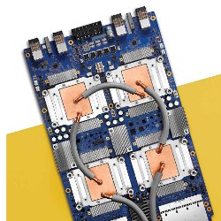
Figure. Google’s Tensor Processing Unit 3.0, introduced last May, is eight times more powerful than 2.0, with performance up to 100 petaflops.
Domain-specific architectures for DNNs continue to be a hot topic among computer architects. A major focus is architectures for sparse matrices, which appeared after the TPU was first deployed in 2015. The Efficient Inference Engine is based on a first pass that reduces the number of weights by approximately a factor of 1013 as a separate step by filtering out very small values and then uses Huffman encoding to shrink the data even further to improve inference performance.14 Cnvlutin1 avoids multiplications when an activation input is zero, as it is 44% of the time, presumably in part due to rectified linear unit, or ReLU, nonlinear function that transforms negative values to zero, improving performance by an average 1.4x. Eyeriss is a novel, low-power dataflow architecture that takes advantage of zeros through run-length encoding data to reduce the memory footprint and saves power by avoiding computations when an input is zero.8 Minerva is a co-design system that crosses algorithm, architecture, and circuit disciplines to reduce power by 8× by in part pruning activation data with small values and in part quantizing the data.31 That effort reported in 2017 is SCNN,27 an accelerator for sparse and compressed convolutional neural networks (CNNs). Both weights and activations are kept compressed in DRAM and in internal buffers, thus shrinking the time and energy needed for data transfers and allowing the chip to store larger models.
Another trend since 2016 is domain-specific architectures for training. For example, ScaleDeep35 is an investigation of a high-performance server designed for DNN training and inference containing thousands of processors. Each chip would contain compute-heavy blocks and memory-heavy blocks, in a 3:1 ratio, and outperform GPUs by 6× to 28×. It computes in 16-bit or 32-bit floating-point arithmetic. The chips are connected through a high-performance interconnect topology that matches DNN communication patterns. Like SCNN, such topologies are evaluated exclusively on CNNs. CNNs were just 5% of the TPU workload in Google’s datacenters in 2016. Computer architects look forward to evaluation of ScaleDeep on other types of DNNs and to hardware implementations.
DNNs would seem to be a good use case for FPGAs as a compute platform in datacenters. The one deployed example is Catapult.30 Although publicly announced in 2014, Catapult is a TPU contemporary since it deployed 28nm Stratix V FPGAs into Microsoft datacenters concurrently with the TPU in 2015. Catapult runs CNNs 2.3× faster than a server. Perhaps the most significant difference between Catapult and the TPU is that to achieve best performance, users must write long programs in the low-level hardware-design-language Verilog vs. writing short programs using the high-level TensorFlow framework; that is, “re-programmability” comes from software for the TPU rather than from firmware for the fastest FPGA.
Conclusion
Despite living on an I/O bus and having relatively limited memory bandwidth constraining utilization of the TPU (four of the six DNN applications are memory-bound), a small fraction of a big number—65,536 multiply-accumulates per cycle—can nonetheless be relatively large, as demonstrated by the Roofline performance model. This result suggests a “cornucopia corollary” to Amdahl’s Law—that low utilization of a huge, cheap resource can still deliver high, cost-effective performance.
We learned that inference applications have serious response-time bounds because they are often part of user-facing applications; DNN architectures thus need to perform well when coping with 99th percentile latency deadlines.
The TPU die leverages its advantage in MACs and on-chip memory to run short programs written using the domain-specific TensorFlow framework 15× faster than the K80 GPU die, resulting in a performance/Watt advantage of 29x, which is correlated with performance/total cost of ownership. Compared to the Haswell CPU die, the corresponding ratios are 29 and 83, respectively.
Five architectural factors explain this energy-performance gap:
One processor. The TPU has only one processor, while the K80 has 13 and the CPU has 18; a single-thread makes it easier for the system to stay within a fixed latency limit;
Large, two-dimensional multiply unit. The TPU has one very large, two-dimensional multiply unit, while the CPU and GPU have 18 and 13 smaller, one-dimensional multiply units, respectively; matrix multiplies benefit from two-dimensional hardware;
Systolic arrays. The two-dimensional organization enables systolic arrays, reducing register accesses and energy;
Eight-bit integers. The TPU’s applications use eight-bit integers rather than 32-bit floating point operations to improve efficiency of both computation and memory; and
Dropped features. The TPU drops features required by CPUs and GPUs that DNNs do not use, making the TPU cheaper while saving energy and allowing transistors to be repurposed for domain-specific on-chip memory.
While future CPUs and GPUs will surely run inference faster, a redesigned TPU using circa-2015 GPU memory would go three times faster and boost the performance/Watt advantage to nearly 70× over the K80 and 200× over Haswell.
For at least the past decade, computer architecture researchers have been publishing innovations based on simulations using limited benchmarks claiming improvements for general-purpose processors of 10% or less, while we are now reporting gains for a domain-specific architecture deployed in real hardware running genuine production applications of more than a factor of 10.17
Order-of-magnitude differences between commercial products are rare in computer architecture, which could even lead to the TPU becoming an archetype for future work in the field. We expect that many will build successors that will raise the bar even higher.
Acknowledgments
We would like to thank all the members of the TPU team for their contributions throughout this project.20 It really does take a village to design, verify, and implement the hardware and software of a system like a TPU and to manufacture, deploy, and use it at scale, as we see at Google.

Figure. Watch the authors discuss their work in this exclusive Communications video. https://cacm.acm.org/videos/a-domain-specific-architecture-for-deep-neural-networks
Sidebar: Energy Proportionality
Thermal design power (TDP) affects the cost of provisioning power, as datacenters must supply sufficient power and cooling when hardware operates at full power. However, the cost of electricity is based on the average consumed as the workload varies during the day. Barroso and Hölzle4 found servers are 100% busy less than 10% of the time and thus advocated energy proportionality, arguing that servers should consume power proportional to the amount of work performed. The estimate of power consumed in Figure 4 is based on the fraction of the TDP seen in Google datacenters.
We measured performance and power of the three servers running the production program CNN0, as the offered workload utilization varies, then normalized to the number of chips per server.
The sidebar figure shows the TPU has the lowest power—40W per chip—but has poor energy proportionality. (Google’s short TPU design schedule prevented inclusion of many energy-saving features.) The Haswell CPU had the best energy proportionality in 2016. In a combined TPU-Haswell system, CPU workload is reduced and thus so is CPU power. Consequently, the Haswell server plus four low-power TPUs uses less than 20% additional power but runs CNN0 80× faster than the Haswell server alone, as it has four TPUs vs. two CPUs.

Figure. The TPU has the lowest power but also poor energy proportionality.


Join the Discussion (0)
Become a Member or Sign In to Post a Comment